IMDB Exploratory Analysis (Python & SQL)

This project is about the exploratory analysis of the IMDb databank, the world’s most popular and authoritative source for movie, TV and celebrity content.
This was a project taught on a free course I signed called “Python Fundamentos Para Análise de Dados 3.0” from the Data Science Academy, and I enjoyed it so much because it focused a lot on data munging and graph production. Thus, I saw it was important to post my step by step records, so I can come back to reuse some useful code and maybe it can teach a curious viewer.
Without further due, we are going to use some SQL knowledge and a lot of Python, focused on data analysis.
When we talk about exploratory analysis, it’s usual to gather a few questions we want to clarify. Thus, what questions could you ask from a movie database IMDB?
What are the most common movies?
What is the number of titles by genre?
The median movie rating by genre and year of release?
The film with the longer duration?
Relationship between duration and gender?
Movies produced by country?
The top 10? worst 10?
So let’s start looking for them.
from platform import python_version
print(python_version())
3.8.8
!pip install -q imdb-sqlite
Now we run the package for downloading the datasets from the site
# https://pypi.org/project/pycountry/

!pip install -q pycountry
Importing other usual packages
import re #regular expressions, text processing
import time #shows execution time
import sqlite3 #manipulate sqlite
import pycountry
import numpy as np
import pandas as pd
import matplotlib.pyplot as plt
import seaborn as sns
from matplotlib import cm
from sklearn.feature_extraction.text import CountVectorizer #vector generator to make calculations
import warnings
warnings.filterwarnings("ignore")
sns.set_theme(style="whitegrid")
Loading data: Downloading from site (take a long time: mine took 50min :()
%%time
!imdb-sqlite
Wall time: 31min 18s


2021-11-26 10:41:30,329 GET https://datasets.imdbws.com/name.basics.tsv.gz -> downloads\name.basics.tsv.gz
2021-11-26 10:42:09,495 GET https://datasets.imdbws.com/title.basics.tsv.gz -> downloads\title.basics.tsv.gz
2021-11-26 10:42:35,228 GET https://datasets.imdbws.com/title.akas.tsv.gz -> downloads\title.akas.tsv.gz
2021-11-26 10:43:19,439 GET https://datasets.imdbws.com/title.principals.tsv.gz -> downloads\title.principals.tsv.gz
2021-11-26 10:44:26,200 GET https://datasets.imdbws.com/title.episode.tsv.gz -> downloads\title.episode.tsv.gz
2021-11-26 10:44:32,314 GET https://datasets.imdbws.com/title.ratings.tsv.gz -> downloads\title.ratings.tsv.gz
2021-11-26 10:44:33,488 Populating database: imdb.db
2021-11-26 10:44:33,489 Applying schema
2021-11-26 10:44:33,500 Importing file: downloads\name.basics.tsv.gz
2021-11-26 10:44:33,500 Reading number of rows ...
2021-11-26 10:44:39,672 Inserting rows into table: people
...
#Conecting to the DB
conn = sqlite3.connect("imdb.db")
#Extract the table list
tables = pd.read_sql_query("SELECT NAME AS 'Table_Name' FROM sqlite_master WHERE type = 'table'",conn)

# The upper words are SQL syntax and the lower are the ones we are searching on the DB

# We make a query
# select name as = alias created
# from sqlite master catalog
# table type filtered
type(tables)
pandas.core.frame.DataFrame
tables.head()

Table_Name
0	people
1	titles
2	akas
3	crew
4	episodes
# Convert df into list
tables = tables["Table_Name"].values.tolist()
# Run the table list at the db and extract the scheme (details) from each one

for table in tables:
    query = "PRAGMA TABLE_INFO({})".format(table)
    result = pd.read_sql_query(query,conn)
    print("Table:", table)
    display(result)
    print("-"*100)
    print("\n") #pk = primary key

        Table: people
       cid	name	    type	notnull	dflt_value	pk
    0	0	person_id	VARCHAR	    0	    None	1
    1	1	name	    VARCHAR	    0	    None	0
    2	2	born	    INTEGER	    0	    None	0
    3	3	died	    INTEGER	    0	    None	0
----------------------------------------------------------------------------------------------------


        Table: titles
        cid	        name	    type	  notnull	dflt_value	pk
    0	0	title_id	        VARCHAR	    0	    None	    1
    1	1	type	            VARCHAR	    0	    None	    0
    2	2	primary_title	    VARCHAR	    0	    None	    0
    3	3	original_title	    VARCHAR	    0	    None	    0
    4	4	is_adult	        INTEGER	    0	    None	    0
    5	5	premiered	        INTEGER	    0	    None	    0
    6	6	ended	            INTEGER	    0	    None	    0
    7	7	runtime_minutes     INTEGER	    0	    None	    0
    8	8	genres	            VARCHAR	    0	    None	    0
----------------------------------------------------------------------------------------------------


        Table: akas
    cid	    name	            type	            notnull	    dflt_value	      pk
0	0	title_id	            VARCHAR 	            0	        None	       0
1	1	title	                VARCHAR 	            0	        None	       0
2	2	region	                VARCHAR 	            0	        None	       0
3	3	language	            VARCHAR	            0	        None	       0
4	4	types	                VARCHAR	            0	        None	       0
5	5	attributes	            ARCHAR	            0	        None	       0
6	6	is_original_title	    INTEGER	            0	        None	       0
----------------------------------------------------------------------------------------------------


Table: crew
    cid	   name	        type	      notnull 	    dflt_value      pk
0	0	title_id	    VARCHAR	        0	            None	        0
1	1	person_id	    VARCHAR	        0	            None	        0
2	2	category	    VARCHAR	        0	            None	        0
3	3	job	            VARCHAR	        0	            None	        0
4	4	characters	    VARCHAR	        0	            None	        0
----------------------------------------------------------------------------------------------------


Table: episodes
cid	     name	                type	 notnull      dflt_value         pk
0	    episode_title_id         INTEGER     0         None            0
1	    show_title_id	        INTEGER	    0	     None	         0
2	    season_number	        INTEGER	    0	     None	         0
3	    eposide_number	        INTEGER	    0	     None	         0
----------------------------------------------------------------------------------------------------


Table: ratings
    cid	    name	type	notnull	dflt_value	pk
0	 0	title_id	VARCHAR	  0	     None	    1
1	 1	rating	    INTEGER	  0	     None	    0
2	 2	votes	    INTEGER	  0	     None	    0
----------------------------------------------------------------------------------------------------
Exploratory Analysis
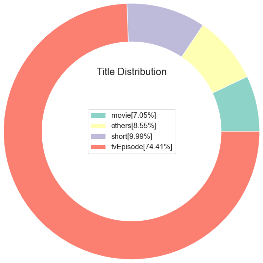
Which are the main types (categories) from the titles (movies)?
#Create the SQL query
query1 =  '''SELECT type, COUNT(*) AS COUNT FROM titles GROUP BY type'''

# SELCT the category
# COUNT = register number
# FROM titles table
# GROUP BY type = cluster for type

# How do I know which table to query? I must seek in the doc
#Result extracting

result1 = pd.read_sql_query(query1, conn) #make the query on my open conection conn
display(result1)

    type	            COUNT
0	movie	            594996
1	short	            843498
2	tvEpisode	        6282068
3	tvMiniSeries	    40802
4	tvMovie	            133772
5	tvPilot	            2
6	tvSeries	        216832
7	tvShort	            10366
8	tvSpecial	        34958
9	video	            254872
10	videoGame	        29785
# Lets calculate the percentual for each type
result1["percentage"] = (result1["COUNT"]/result1["COUNT"].sum())*100

# each category total from the COUNT table and divide it by the COUNT records sum
display(result1)

    type	        COUNT	percentual
0	movie	        594996	 7.048086
1	short	        843498	 9.991742
2	tvEpisode	   6282068	74.414883
3	tvMiniSeries	 40802	 0.483324
4	tvMovie	        133772	 1.584610
5	tvPilot	             2	 0.000024
6	tvSeries	    216832	 2.568506
7	tvShort	         10366	 0.122792
8	tvSpecial	     34958	 0.414099
9	video	        254872	 3.019113
10	videoGame	     29785	 0.352821
# But what if I just wanna deliver 4 categories:
# The 3 ones with most titles and a last one with all the rest

#Make an empy dict
others={}

#Filter the percentual at 5% and sum the total
others["COUNT"] =  result1[result1["percentage"]<5]["COUNT"].sum()

#Save the percentual
others["percentage"] = result1[result1["percentage"]<5]['percentage'].sum()

#Name adjusting
others["type"] = "others"
others #any category with less than 5% went to the others category
{'COUNT': 721389, 'percentual': 8.545287694752078, 'type': 'others'}
# Filter the result from df

result1 =  result1[result1['percentage']>5]
# Append the top 3 result with the "others": less than 5%

result1 = result1.append(others, ignore_index= True)
# Ordering the result
result1 =  result1.sort_values(by = "COUNT",ascending= True)
result1.head()

    type	    COUNT	 percentual
0	movie	    594996	  7.048086
3	others  	721389	  8.545288
1	short	    843498	  9.991742
2	tvEpisode   6282068   74.414883
#Now lets adjust the labels, that is a list comprehension (in one function a serie of commands)

labels =[str(result1['type'][i])+''+'['+str(round(result1['percentage'][i],2))+"%"+"]" for i in result1.index]
#Plot

# We can see some parameters to make it on our own style at matplot colormap tips

cs= cm.Set3(np.arange(100))

#Make the figure
f = plt.figure()

# Pie Plot

plt.pie(result1["COUNT"], labeldistance=1, radius=3, colors=cs, wedgeprops= dict(width=0.9))
plt.legend(labels=labels,loc="center",prop={"size":15})
plt.title("Title Distribution", loc = "Center",fontdict = {"fontsize":20,"fontweight":30})
plt.show
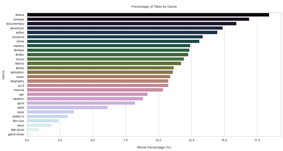
What is the number of titles by genre?
1º calculate the number of movies by genre
2º deliver the result in percentual
# Create the SQL query

query2 =  '''SELECT genres, COUNT(*) FROM titles WHERE type = "movie" GROUP BY genres'''
result2 = pd.read_sql_query(query2,conn)
display(result2)
# Convert the strings from upper to lower case

result2["genres"] = result2["genres"].str.lower().values
#Removing NA values

temp = result2["genres"].dropna()
Now we must try to find a way to count the number of movies for each genre
Count Vectorizer (Sparse matrix)
It is used to transform a given text into a vector (one-hot-encoded) on the basis of the frequency (count) of each word that occurs in the entire text. It involves counting the number of occurences each words appears in a document (text).
The result of this method is a Sparse matrix.They are matrices in which most positions are filled with zeros. For these arrays, we can save significant memory space if only nonzero terms are stored.
Ex:
Movies --> Terror  Romance  Action

Horror        1       0        0
Action        0       0        1
Romance       0       1        0
Horror        1       0        0
#So now we are gonna create a vector using the regular expression to filter the strings
# We can search html re strings on python library

usual = "(?u)\\b[\\w-]+\\b"

vector = CountVectorizer(token_pattern = usual, analyzer="word").fit(temp)
type(vector)
sklearn.feature_extraction.text.CountVectorizer
#Apply the vectorization to the df

matrix = vector.transform(temp)
type(matrix)
scipy.sparse.csr.csr_matrix
#Returning unique genres

unique_genres = vector.get_feature_names()
unique_genres
['action',
 'adult',
 'adventure',
 'animation',
 'biography',
 'comedy',
 'crime',
 'documentary',
 'drama',
 'family',
 'fantasy',
 'film-noir',
 'game-show',
 'history',
 'horror',
 'music',
 'musical',
 'mystery',
 'n',
 'news',
 'reality-tv',
 'romance',
 'sci-fi',
 'short',
 'sport',
 'talk-show',
 'thriller',
 'war',
 'western']
genres = pd.DataFrame(matrix.todense(),columns=unique_genres,index= temp.index)
genres.info()
<class 'pandas.core.frame.DataFrame'>
Int64Index: 1451 entries, 0 to 1450
Data columns (total 29 columns):
 #   Column       Non-Null Count  Dtype
---  ------       --------------  -----
 0   action       1451 non-null   int64
 1   adult        1451 non-null   int64
 2   adventure    1451 non-null   int64
 3   animation    1451 non-null   int64
 4   biography    1451 non-null   int64
 5   comedy       1451 non-null   int64
 6   crime        1451 non-null   int64
 7   documentary  1451 non-null   int64
 8   drama        1451 non-null   int64
 9   family       1451 non-null   int64
 10  fantasy      1451 non-null   int64
 11  film-noir    1451 non-null   int64
 12  game-show    1451 non-null   int64
 13  history      1451 non-null   int64
 14  horror       1451 non-null   int64
 15  music        1451 non-null   int64
 16  musical      1451 non-null   int64
 17  mystery      1451 non-null   int64
 18  n            1451 non-null   int64
 19  news         1451 non-null   int64
 20  reality-tv   1451 non-null   int64
 21  romance      1451 non-null   int64
 22  sci-fi       1451 non-null   int64
 23  short        1451 non-null   int64
 24  sport        1451 non-null   int64
 25  talk-show    1451 non-null   int64
 26  thriller     1451 non-null   int64
 27  war          1451 non-null   int64
 28  western      1451 non-null   int64
dtypes: int64(29)
memory usage: 340.1 KB
#Drop the n column

genres = genres.drop(columns="n",axis=0)
#Calculating the percentual

genres_percentage = 100*pd.Series(genres.sum()).sort_values(ascending = False)/genres.shape[0]
genres_percentage.head()
drama          18.401103
comedy         16.884907
documentary    15.920055
adventure      14.886285
action         14.472777
dtype: float64
# Plot

plt.figure(figsize = (16,8))
sns.barplot(x = genres_percentual.values, y = genres_percentual.index, orient="h", palette = "cubehelix")
plt.ylabel("Genre")
plt.xlabel("\nMovie Percentage (%)")
plt.title("\nPercentage of Titles by Genre\n")
plt.show()
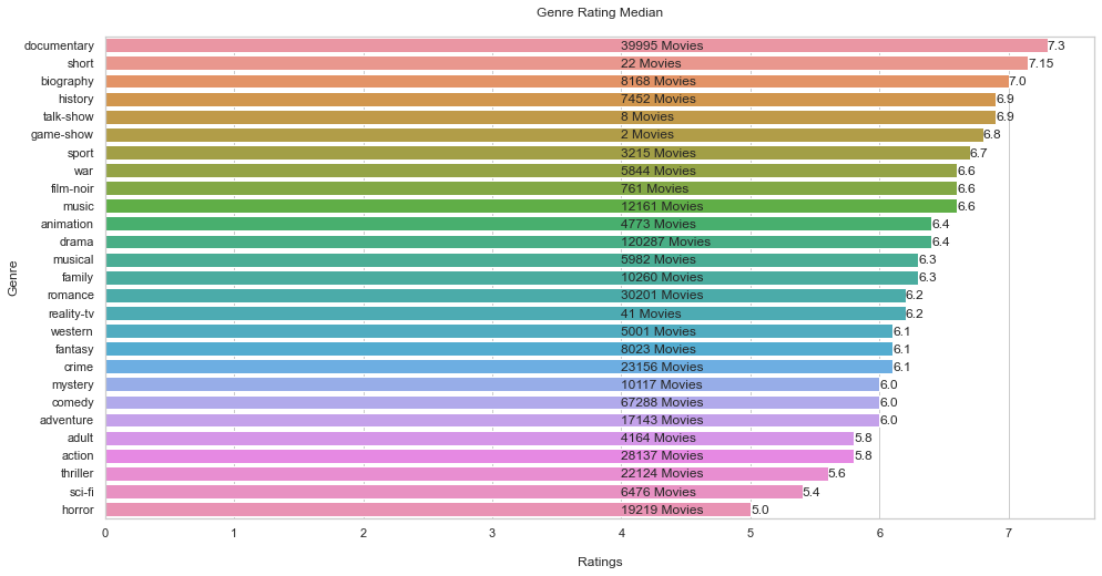
What is the median of ratings by gender?
Why median and not the mean?
Mean = affected by outliers
Median = is not affected by outliers, safer
# Query

query3 ='''
        SELECT rating, genres FROM
        ratings JOIN titles ON ratings.title_id = titles.title_id
        WHERE premiered <= 2022 AND type = 'movie'
        '''
# SELECTING rating and genres from 2 tables (ratings and titles) and joining them
# Then we filter(WHERE, not when) asking what was the year that movie was first released
result3 = pd.read_sql_query(query3, conn)
display(result3)

	  rating	    genres
0	    4.5	        \N
1	    6.1	        Action,Adventure,Biography
2	    5.2	        Drama
3	    4.5	        Drama
4	    3.8	        Drama
...	...	...
271240	3.6	        Action,Adventure,Thriller
271241	5.8	        Thriller
271242	6.4	        Drama,History
271243	3.8	        Adventure,History,War
271244	8.3	        Drama

271245 rows × 2 columns
# Now lets create a function to return the genres

def genres_return(df):
    df['genres']= df['genres'].str.lower().values
    temp = df['genres'].dropna()
    vector= CountVectorizer(token_pattern="(?u)\\b[\\w-]+\\b",analyzer="word").fit(temp)
    unique_genre = vector.get_feature_names()
    unique_genre = [genre for genre in unique_genre if len(genre)>1]
    return unique_genre
unique_genres= genres_return(result3)
unique_genres
['action',
 'adult',
 'adventure',
 'animation',
 'biography',
 'comedy',
 'crime',
 'documentary',
 'drama',
 'family',
 'fantasy',
 'film-noir',
 'game-show',
 'history',
 'horror',
 'music',
 'musical',
 'mystery',
 'news',
 'reality-tv',
 'romance',
 'sci-fi',
 'short',
 'sport',
 'talk-show',
 'thriller',
 'war',
 'western']
#Create empty lists to make the count
genre_counts =[]
genre_ratings =[]
for item in unique_genres:

    #Return the movie count by genres
    query = 'SELECT COUNT(rating) FROM ratings JOIN titles ON ratings.title_id=titles.title_id WHERE genres LIKE '+ '\''+'%'+item+'%'+'\' AND type=\'movie\''
    result = pd.read_sql_query(query,conn)
    genre_counts.append(result.values[0][0])

    #return the ratings by genre
    query =  'SELECT rating FROM ratings JOIN titles ON ratings.title_id=titles.title_id WHERE genres LIKE '+ '\''+'%'+item+'%'+'\' AND type=\'movie\''
    result = pd.read_sql_query(query,conn)
    genre_ratings.append(np.median(result["rating"])) #calculating the median
# Preparing the final df

df_genre_ratings = pd.DataFrame()
df_genre_ratings['genres'] = unique_genres
df_genre_ratings['count'] = genre_counts
df_genre_ratings['rating'] = genre_ratings
df_genre_ratings.head(20)

    genres	    count	rating
0	action	    28137	 5.8
1	adult	     4164	 5.8
2	adventure	17143	 6.0
3	animation	 4773	 6.4
4	biography	 8168	 7.0
5	comedy	    67288	 6.0
6	crime	    23156	 6.1
7	documentary	39995	 7.3
8	drama	   120287	 6.4
9	family	    10260	 6.3
10	fantasy	     8023	 6.1
11	film-noir	  761	 6.6
12	game-show	    2	 6.8
13	history	     7452	 6.9
14	horror	    19219	 5.0
15	music	    12161	 6.6
16	musical	     5982	 6.3
17	mystery	    10117	 6.0
18	news	      664	 7.3
19	reality-tv	   41	 6.2
#Drop the news column

df_genre_ratings = df_genre_ratings.drop(index=18)
#Sorting the result
df_genre_ratings = df_genre_ratings.sort_values(by="rating",ascending=False)
# Plot

plt.figure(figsize = (16,8))
sns.barplot(x = df_genre_ratings.rating, y = df_genre_ratings.genres, orient="h")

# Graphic text
for i in range(len(df_genre_ratings.index)):

    plt.text(4.0,
             i + 0.25,
             str(df_genre_ratings['count'][df_genre_ratings.index[i]]) + " Movies")

    plt.text(df_genre_ratings.rating[df_genre_ratings.index[i]],
             i + 0.25,
             round(df_genre_ratings["rating"][df_genre_ratings.index[i]],2))


plt.ylabel("Genre")
plt.xlabel("\nRatings")
plt.title('Genre Rating Median\n')
plt.show()

# Without each movies total, the info could be biased.
# Look at the top 2 ratings and the total of each one.
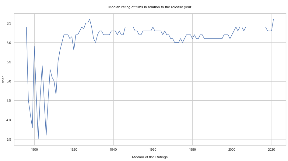
What is the median rating of movies in relation to the release year?
query4 ='''
        SELECT rating as Ratings, premiered FROM
        ratings JOIN titles ON ratings.title_id = titles.title_id
        WHERE premiered <= 2022 AND type = 'movie'
        ORDER by premiered'''


# on the oficial doc there is a column called premiered that contains the year each movie was released
# it is always important to query the raw info
result4 = pd.read_sql_query(query4,conn)
display(result4)

    Ratings	   premiered
0	    6.4	    1896
1	    4.5	    1897
2	    3.9	    1899
3	    3.7	    1899
4	    6.0	    1900
...	...	...
271240	8.6	    2021
271241	7.7	    2021
271242	5.6	    2021
271243	6.0	    2021
271244	8.2	    2021

271245 rows × 2 columns
#Calculate the median over time

ratings = []
for year in set(result4["premiered"]):
    ratings.append(np.median(result4[result4["premiered"]==year]['Ratings']))

#We are going to travel each year for each movie, and then calculate the median
years = list(set(result4['premiered']))
# Plot

plt.figure(figsize = (16,8))
plt.plot(years,ratings)
plt.ylabel("Year")
plt.xlabel("\nMedian of the Ratings")
plt.title("\nMedian rating of films in relation to the release year\n")
plt.show()
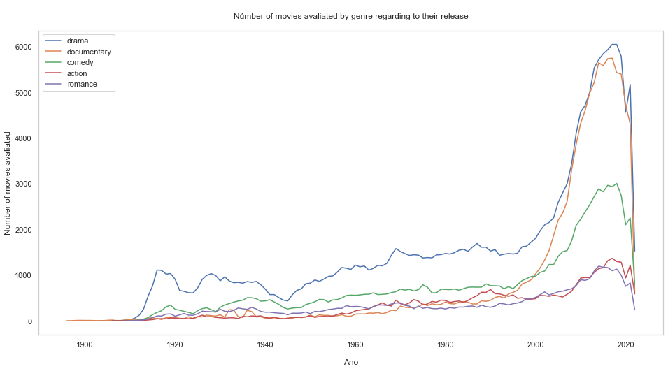
What is the number of movies rated by genre regarding to the release year?
query5= '''SELECT genres FROM titles'''
result5 = pd.read_sql_query(query5,conn)
display(result5)

                genres
0	        Documentary,Short
1	        Animation,Short
2	        Animation,Comedy,Romance
3	        Animation,Short
4	        Comedy,Short
...	...
8441946	    Action,Drama,Family
8441947	    Action,Drama,Family
8441948	    Action,Drama,Family
8441949	    Short
8441950	    Adventure,Animation,Comedy

8441951 rows × 1 columns
#Returning single genre, I guess it suits better than unique XD

single_genre = genres_return(result5)
#Now we count

genre_count = []

for item in single_genre:
    query = 'SELECT COUNT(*) COUNT FROM  titles  WHERE genres LIKE '+ '\''+'%'+item+'%'+'\' AND type=\'movie\' AND premiered <= 2022'
    result = pd.read_sql_query(query, conn)
    genre_count.append(result['COUNT'].values[0])
#Preparing the df
df_genre_count = pd.DataFrame()
df_genre_count['genre']= single_genre
df_genre_count['count']= genre_count
# Calculating the top 5
df_genre_count = df_genre_count[df_genre_count['genre'] != 'n'] #everything that isn't n
df_genre_count = df_genre_count.sort_values(by = 'count', ascending = False)
top_genre = df_genre_count.head()['genre'].values
# Plot

# Fig
plt.figure(figsize = (16,8))

# Loop and Plot
for item in top_genre:
    query = 'SELECT COUNT(*) Number_of_movies, premiered Year FROM  titles  WHERE genres LIKE '+ '\''+'%'+item+'%'+'\' AND type=\'movie\' AND Year <=2022 GROUP BY Year'
    result = pd.read_sql_query(query, conn)
    plt.plot(result['Year'], result['Number_of_movies'])

plt.grid(b=None)
plt.xlabel('\nAno')
plt.ylabel('Number of movies avaliated')
plt.title('\nNúmber of movies avaliated by genre regarding to their release\n')
plt.legend(labels = top_genre)
plt.show()
What is the longest movie? Compute the Percentis
query6= '''
        SELECT runtime_minutes Runtime
        FROm titles
        WHERE type = "movie" AND Runtime != "NaN"
        '''

#Percentis allow you to divide your data in 100 equal parts
#It is a way to identify outliers. The clusters 1 and 100 may present theses extreme values.
result6 = pd.read_sql_query(query6,conn)
display(result6)

        Runtime
0	    100
1	    70
2	    90
3	    120
4	    58
...	...
374083	123
374084	57
374085	100
374086	116
374087	49
# Percentil Loop

for i in range(101):
    val = i
    perc = round(np.percentile(result6["Runtime"].values,val),2)
    print('{} percentil of the duration(runtime)is: {}'.format(val,perc))
0 percentil of the duration(runtime)is: 1.0
1 percentil of the duration(runtime)is: 45.0
2 percentil of the duration(runtime)is: 48.0
3 percentil of the duration(runtime)is: 50.0
4 percentil of the duration(runtime)is: 50.0
5 percentil of the duration(runtime)is: 52.0
6 percentil of the duration(runtime)is: 52.0
7 percentil of the duration(runtime)is: 54.0
8 percentil of the duration(runtime)is: 55.0
9 percentil of the duration(runtime)is: 56.0
10 percentil of the duration(runtime)is: 58.0
11 percentil of the duration(runtime)is: 59.0
12 percentil of the duration(runtime)is: 60.0
13 percentil of the duration(runtime)is: 60.0
14 percentil of the duration(runtime)is: 60.0
15 percentil of the duration(runtime)is: 62.0
16 percentil of the duration(runtime)is: 63.0
17 percentil of the duration(runtime)is: 65.0
18 percentil of the duration(runtime)is: 66.0
19 percentil of the duration(runtime)is: 68.0
20 percentil of the duration(runtime)is: 70.0
21 percentil of the duration(runtime)is: 70.0
22 percentil of the duration(runtime)is: 71.0
23 percentil of the duration(runtime)is: 72.0
24 percentil of the duration(runtime)is: 73.0
25 percentil of the duration(runtime)is: 74.0
26 percentil of the duration(runtime)is: 75.0
27 percentil of the duration(runtime)is: 75.0
28 percentil of the duration(runtime)is: 76.0
29 percentil of the duration(runtime)is: 77.0
30 percentil of the duration(runtime)is: 78.0
31 percentil of the duration(runtime)is: 79.0
32 percentil of the duration(runtime)is: 80.0
33 percentil of the duration(runtime)is: 80.0
34 percentil of the duration(runtime)is: 80.0
35 percentil of the duration(runtime)is: 81.0
36 percentil of the duration(runtime)is: 82.0
37 percentil of the duration(runtime)is: 82.0
38 percentil of the duration(runtime)is: 83.0
39 percentil of the duration(runtime)is: 84.0
40 percentil of the duration(runtime)is: 84.0
41 percentil of the duration(runtime)is: 85.0
42 percentil of the duration(runtime)is: 85.0
43 percentil of the duration(runtime)is: 85.0
44 percentil of the duration(runtime)is: 86.0
45 percentil of the duration(runtime)is: 86.0
46 percentil of the duration(runtime)is: 87.0
47 percentil of the duration(runtime)is: 87.0
48 percentil of the duration(runtime)is: 88.0
49 percentil of the duration(runtime)is: 88.0
50 percentil of the duration(runtime)is: 89.0
51 percentil of the duration(runtime)is: 90.0
52 percentil of the duration(runtime)is: 90.0
53 percentil of the duration(runtime)is: 90.0
54 percentil of the duration(runtime)is: 90.0
55 percentil of the duration(runtime)is: 90.0
56 percentil of the duration(runtime)is: 90.0
57 percentil of the duration(runtime)is: 90.0
58 percentil of the duration(runtime)is: 91.0
59 percentil of the duration(runtime)is: 91.0
60 percentil of the duration(runtime)is: 92.0
61 percentil of the duration(runtime)is: 92.0
62 percentil of the duration(runtime)is: 93.0
63 percentil of the duration(runtime)is: 93.0
64 percentil of the duration(runtime)is: 94.0
65 percentil of the duration(runtime)is: 94.0
66 percentil of the duration(runtime)is: 95.0
67 percentil of the duration(runtime)is: 95.0
68 percentil of the duration(runtime)is: 96.0
69 percentil of the duration(runtime)is: 96.0
70 percentil of the duration(runtime)is: 97.0
71 percentil of the duration(runtime)is: 98.0
72 percentil of the duration(runtime)is: 98.0
73 percentil of the duration(runtime)is: 99.0
74 percentil of the duration(runtime)is: 100.0
75 percentil of the duration(runtime)is: 100.0
76 percentil of the duration(runtime)is: 100.0
77 percentil of the duration(runtime)is: 101.0
78 percentil of the duration(runtime)is: 102.0
79 percentil of the duration(runtime)is: 103.0
80 percentil of the duration(runtime)is: 104.0
81 percentil of the duration(runtime)is: 105.0
82 percentil of the duration(runtime)is: 106.0
83 percentil of the duration(runtime)is: 107.0
84 percentil of the duration(runtime)is: 108.0
85 percentil of the duration(runtime)is: 110.0
86 percentil of the duration(runtime)is: 110.0
87 percentil of the duration(runtime)is: 112.0
88 percentil of the duration(runtime)is: 115.0
89 percentil of the duration(runtime)is: 116.0
90 percentil of the duration(runtime)is: 119.0
91 percentil of the duration(runtime)is: 120.0
92 percentil of the duration(runtime)is: 122.0
93 percentil of the duration(runtime)is: 126.0
94 percentil of the duration(runtime)is: 130.0
95 percentil of the duration(runtime)is: 135.0
96 percentil of the duration(runtime)is: 139.0
97 percentil of the duration(runtime)is: 145.0
98 percentil of the duration(runtime)is: 153.0
99 percentil of the duration(runtime)is: 168.0
100 percentil of the duration(runtime)is: 51420.0
This analysis showed us that our data do have outliers, as we see on the 1 and 100 clusters. It doesn’t mean that these outliers are errors.
query6 = '''
            SELECT runtime_minutes Runtime, primary_title
            FROM titles
            WHERE type = 'movie' AND Runtime != 'NaN'
            ORDER BY Runtime DESC
            LIMIT 1
            '''

# Im going to grab runtime_minutes (as Runtime) and primary_title from titles
# The type is Movie, different from NaN
# Order by the Runtime column in descending order
# Limit = 1 to bring the first record
result6 = pd.read_sql_query(query6,conn)
result6

    Runtime	   primary_title
0	51420	    Logistics
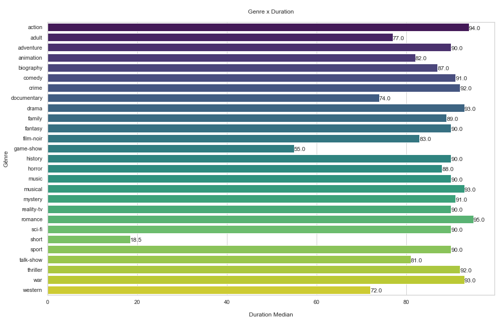
What is the relationship between genre and duration?
query7 = '''
         SELECT AVG(runtime_minutes) Runtime, genres
         FROM titles
         WHERE type = "movie"
         AND runtime_minutes != "NaN"
         GROUP BY genres
         '''
# Call avg function on the runtime_minutes columns by the nickname Runtime
result7= pd.read_sql_query(query7, conn)
single_genres = genres_return(result7) #returning single genres
single_genres
['action',
 'adult',
 'adventure',
 'animation',
 'biography',
 'comedy',
 'crime',
 'documentary',
 'drama',
 'family',
 'fantasy',
 'film-noir',
 'game-show',
 'history',
 'horror',
 'music',
 'musical',
 'mystery',
 'news',
 'reality-tv',
 'romance',
 'sci-fi',
 'short',
 'sport',
 'talk-show',
 'thriller',
 'war',
 'western']
# Calculating duration by genre
genre_runtime = []
for item in single_genres:
    query = 'SELECT runtime_minutes Runtime FROM  titles  WHERE genres LIKE '+ '\''+'%'+item+'%'+'\' AND type=\'movie\' AND Runtime!=\'NaN\''
    result = pd.read_sql_query(query, conn)
    genre_runtime.append(np.median(result['Runtime']))
#Preparing the df

df_genre_runtime = pd.DataFrame()
df_genre_runtime["genre"] = single_genre
df_genre_runtime["runtime"]= genre_runtime
# Removing index 18 (news), we know he has NaN

df_genre_runtime=df_genre_runtime.drop(index=18)
# Plot

# Fig size
plt.figure(figsize = (16,10))

# Barplot
sns.barplot(y = df_genre_runtime.genre, x = df_genre_runtime.runtime, orient = "h", palette="viridis")

# Loop
for i in range(len(df_genre_runtime.index)):
    plt.text(df_genre_runtime.runtime[df_genre_runtime.index[i]],
             i + 0.25,
             round(df_genre_runtime["runtime"][df_genre_runtime.index[i]], 2))

plt.ylabel('Gênre')
plt.xlabel('\nDuration Median')
plt.title('\nGenre x Duration\n')
plt.show()
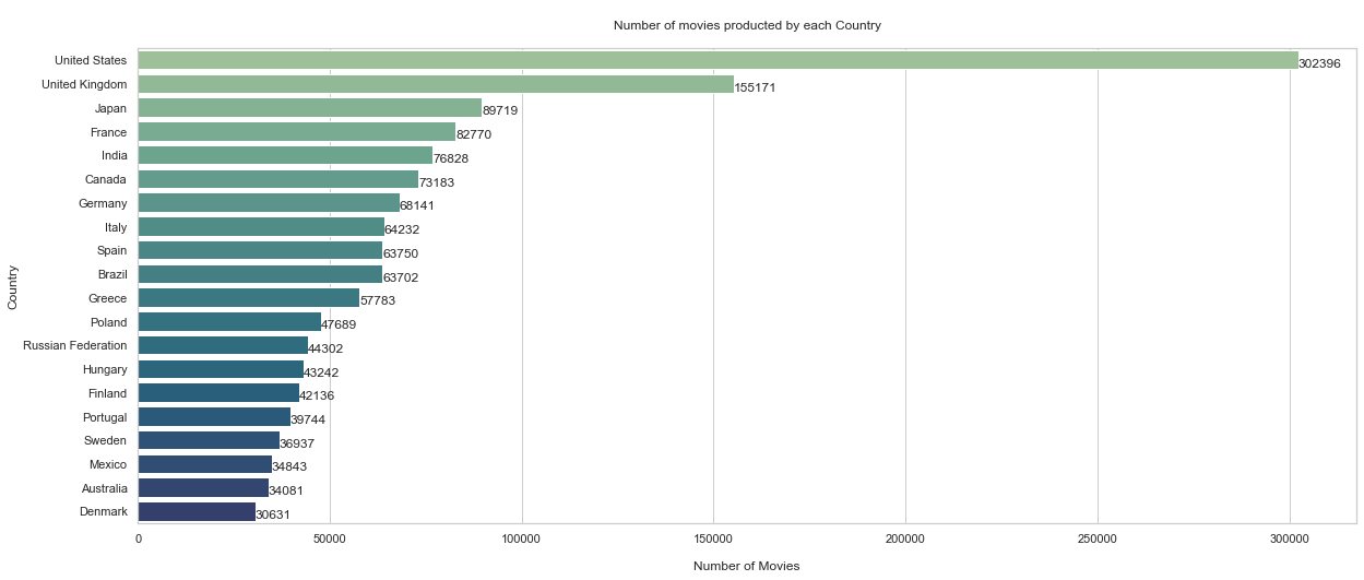
What is the amount of movies made by country?
query8 = '''
         SELECT region, COUNT(*) Number_of_movies FROM
         akas JOIN titles ON
         akas.title_id = titles.title_id
         WHERE region != 'None'
         AND type = \'movie\'
         GROUP BY region
         '''
# Joining tables akas and titles
result8 =pd.read_sql_query(query8,conn)
display(result8) # country codes appear

region	Number_of_movies
0	AD	      22
1	AE	    2996
2	AF	     109
3	AG	      12
4	AL	    1248
...	...	...
229	YUCS	 147
230	ZA	    3098
231	ZM	      12
232	ZRCD	   2
233	ZW	      49

234 rows × 2 columns
result8.shape
(234, 2)
# Empty variables

country_names =[]
count = []
# Loop to obtain the country according to the region

for i in range(result8.shape[0]):
    try:
        coun = result8['region'].values[i]
        country_names.append(pycountry.countries.get(alpha_2 = coun).name)
        count.append(result8['Number_of_movies'].values[i])
    except:
        continue

# This is also a loop to error treatment
# Preparing the dataframe
df_country_movies = pd.DataFrame()
df_country_movies["country"] = country_names
df_country_movies["Movie_Count"] = count
# Sort the results

df_country_movies = df_country_movies.sort_values(by = 'Movie_Count', ascending = False)
df_country_movies.head(10)

    country	        Movie_Count
199	United States	302396
65	United Kingdom	155171
96	Japan	         89719
63	France	         82770
89	India	         76828
32	Canada	         73183
47	Germany	         68141
93	Italy	         64232
58	Spain	         63750
26	Brazil	         63702
# Plot

# Figure
plt.figure(figsize = (20,8))

# Barplot
sns.barplot(y = df_country_movies[:20].country, x = df_country_movies[:20].Movie_Count, orient = "h", palette = "crest")

# Loop
for i in range(0,20):
    plt.text(df_country_movies.Movie_Count[df_country_movies.index[i]]-1,
             i + 0.30,
             round(df_country_movies["Movie_Count"][df_country_movies.index[i]],2))

plt.ylabel('Country')
plt.xlabel('\nNumber of Movies')
plt.title('\nNumber of movies producted by each Country\n')
plt.show()
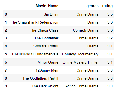
Now the best one: according to the site, which are the top 10 movies?
query9 = '''
            SELECT primary_title AS Movie_Name, genres, rating
            FROM
            titles JOIN ratings
            ON  titles.title_id = ratings.title_id
            WHERE titles.type = 'movie' AND ratings.votes >= 25000
            ORDER BY rating DESC
            LIMIT 10
            '''

# Select primary... as nickname Movie_name
# genres and rating from Titles table
# and joining to the ratings table
# where titles.type are going to be called movie and the only the ones with rating number > 25k

#If I was seeking the 10 worst I would switch DESC for ASC
top10 = pd.read_sql_query(query9,conn)
display(top10)
Now we arrived to the end of this project. This is a very didactic material and I enjoyed so much. I expect you also had a great learnign about that, like I did ;)