Natural Language Processing with Disaster Tweets

Twitter has become an important communication channel in times of emergency. The ubiquitousness of smartphones enables people to announce an emergency they’re observing in real-time. Because of this, more agencies are interested in programmatically monitoring Twitter (i.e. disaster relief organizations and news agencies).
But, it’s not always clear whether a person’s words are announcing a disaster.
Take this example: “Looked at the sky at night yesterday, it was ablaze”.
The author explicitly uses the word “ABLAZE” but means it metaphorically. This is clear to a human right away, especially with the visual aid. But it’s less clear to a machine. In this competition, you’re challenged to build a machine learning model that predicts which Tweets are about real disasters and which ones aren’t. You’ll have access to a dataset of 10,000 tweets that were hand classified.
So, let’s start our job calling the first libs:
import numpy as np
import pandas as pd
df_train = pd.read_csv("/tw_files/train.csv")
df_test = pd.read_csv('/tw_files/test.csv')
df_sample = pd.read_csv('sample_submission.csv')
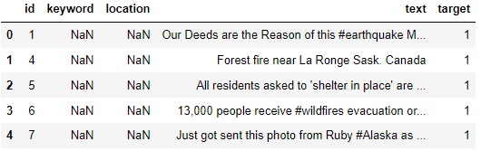
df_train.head(5)
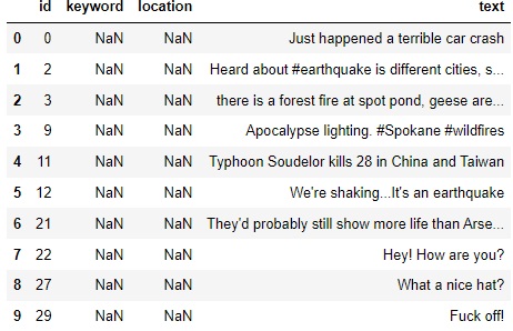
df_test.head(10)
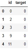
df_sample.head(5)
# Check for null values

df_train.isnull().sum()
df_test.isnull().sum()

    id             0
    keyword       26
    location    1105
    text           0
    dtype: int64
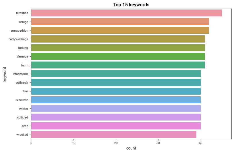
Most common keywords in train dataset
import matplotlib.pyplot as plt import seaborn as sns
sns.set_palette('husl')
plt.figure(figsize=(9,6))
sns.countplot(y = df_train.keyword, order= df_train.keyword.value_counts().iloc[:15].index)
plt.title('Top 15 keywords')
plt.show()
## Plot to checkout null values in train data
df_train.isna().sum().plot(kind = 'bar')
plt.title('Plot to checkout null values in train data')
plt.show()
df_test.isna().sum().plot(kind = 'bar')
plt.title('Plot to checkout null values in test data')
plt.show()
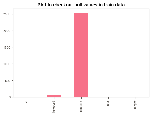
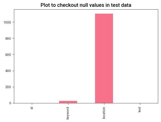
# Since location and keyword have a lot of null values, we can drop them from our data.

df_train = df_train.drop(['location','keyword'],axis=1)
df_test = df_test.drop(['location','keyword'],axis=1)
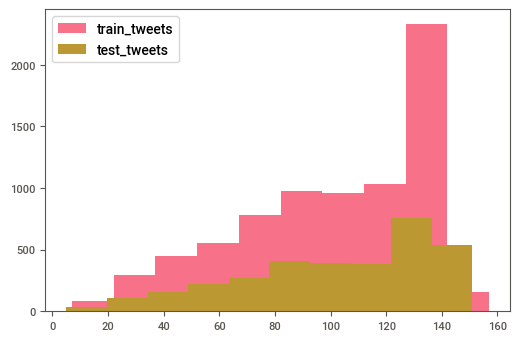
## Plot length of the train and test dataset

plt.hist(df_train['text'].str.len(), label = 'train_tweets')
plt.hist(df_test['text'].str.len(),label = 'test_tweets')
plt.legend()
plt.show()
# We can see that our variable target indicate us what is a disaster tweet (1) and what isn't (0)
# So this is a boolean variable
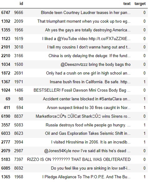
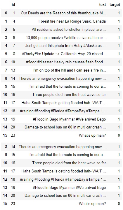
df_train.sample(20)
df_train.head(16)
## Checkout a disaster tweet
d_t = df_train[df_train['target'] == 1]['text'] #Print a text from the range 0-8, if equal to 1
for i in range(0,8):
    print(d_t[i])
Our Deeds are the Reason of this #earthquake May ALLAH Forgive us all
Forest fire near La Ronge Sask. Canada
All residents asked to 'shelter in place' are being notified by officers. No other evacuation or shelter in place orders are expected
13,000 people receive #wildfires evacuation orders in California
Just got sent this photo from Ruby #Alaska as smoke from #wildfires pours into a school
RockyFire Update => California Hwy. 20 closed in both directions due to Lake County fire - #CAfire #wildfires
flood #disaster Heavy rain causes flash flooding of streets in Manitou, Colorado Springs areas
I am on top of the hill and I can see a fire in the woods
## Checkout a non disaster tweet
nd_t = df_train[df_train['target'] != 1]['text'] #Print a text if different from 1
print(nd_t.head(5)) #it starts from 15 because it is the first row to have a 0
15                  What's up man?
16                   I love fruits
17                Summer is lovely
18               My car is so fast
19    What a goooooooaaaaaal!!!!!!
Name: text, dtype: object
nd_t = df_train[df_train['target'] == 1]['text']
print(nd_t.head(5))
0    Our Deeds are the Reason of this #earthquake M...
1               Forest fire near La Ronge Sask. Canada
2    All residents asked to 'shelter in place' are ...
3    13,000 people receive #wildfires evacuation or...
4    Just got sent this photo from Ruby #Alaska as ...
Name: text, dtype: object
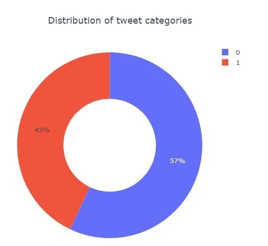
import plotly.express as px
px.pie(df_train,names='target',title='Distribution of tweet categories',hole=0.5)
Data Cleaning
import re
import string
def clean_text(t):
    # Convert to lower
    t = t.lower()
    # remove html tags
    t = re.sub(r'\[.*?\]',' ', t)
    # remove link
    t = re.sub(r'https?://\S+|www\.\S+',' ', t)
    #remove line breaks
    t = re.sub(r'\n',' ',t)
    #Remove trailing spaces, tabs
    t  = re.sub('\s+',' ',t)
    # remove punctuation
#     t = re.sub('[%s]' % re.escape(string.punctuation), t)
    # Remove special characters
    t = re.sub('\w*\d\w*','',t)
    return t

## Apply clean function on random train string
test_str = df_train.loc[417, 'text']
print('Original text: '+test_str+'\n')
print('Original text after cleaning: '+clean_text(test_str))
Original text: Arson suspect linked to 30 fires caught in Northern California http://t.co/mmGsyAHDzb

Original text after cleaning: arson suspect linked to  fires caught in northern california
## Applying clean function on train & test sets
df_train['text'] = df_train['text'].apply(lambda x:clean_text(x))
df_test['text'] = df_test['text'].apply(lambda x:clean_text(x))

## checkout train after cleaning
df_train['text'].head(5)
0    our deeds are the reason of this #earthquake m...
1               forest fire near la ronge sask. canada
2    all residents asked to 'shelter in place' are ...
3    , people receive #wildfires evacuation orders ...
4    just got sent this photo from ruby #alaska as ...
Name: text, dtype: object
Tokenization
A RegexpTokenizer splits a string into substrings using a regular expression. For example, the following tokenizer forms tokens out of alphabetic sequences, money expressions, and any other non-whitespace sequences:
from nltk.tokenize import RegexpTokenizer s = “Good muffins cost $3.88\nin New York. Please buy me\ntwo of them.\n\nThanks.”
tokenizer = RegexpTokenizer('\w+|$[\d.]+|\S+’)
tokenizer.tokenize(s) [‘Good’, ‘muffins’, ‘cost’, ‘in’, ‘New’, ‘York’, ‘.’, ‘Please’, ‘buy’, ‘me’, ‘two’, ‘of’, ‘them’, ‘.’, ‘Thanks’, ‘.']
# Tokenize the cleaned sentences
import nltk
from nltk.corpus import stopwords
from nltk.stem import WordNetLemmatizer
from nltk import RegexpTokenizer

# tokenizer=nltk.tokenize.RegexpTokenizer(r'\w+')
tokenizer = RegexpTokenizer(r'\w+')
## Applying tokenization function on train & test sets
df_train['text'] = df_train['text'].map(tokenizer.tokenize)
df_test['text'] = df_test['text'].map(tokenizer.tokenize) ## checkout train dataset tokens
df_train['text'].head(5)
0    [our, deeds, are, the, reason, of, this, earth...
1        [forest, fire, near, la, ronge, sask, canada]
2    [all, residents, asked, to, shelter, in, place...
3    [people, receive, wildfires, evacuation, order...
4    [just, got, sent, this, photo, from, ruby, ala...
Name: text, dtype: object
Stopwords:
remove unnecessary words that do not carry any meaning
import nltk
#nltk.download('stopwords')

def remove_stopwords(t):
    words = [w for w in t if w not in stopwords.words('english')]
    return words

df_train['text'] =df_train['text'].apply(lambda x: remove_stopwords(x))
df_test['text'] =df_test['text'].apply(lambda x: remove_stopwords(x))

## checkout train dataset without stopwords
df_train['text'].head(5)
[nltk_data] Downloading package stopwords to
[nltk_data]     C:\Users\lucas\AppData\Roaming\nltk_data...
[nltk_data]   Package stopwords is already up-to-date!


0    [deeds, reason, earthquake, may, allah, forgiv...
1        [forest, fire, near, la, ronge, sask, canada]
2    [residents, asked, shelter, place, notified, o...
3    [people, receive, wildfires, evacuation, order...
4    [got, sent, photo, ruby, alaska, smoke, wildfi...
Name: text, dtype: object
Lemmatization
Lemmatization is the process of grouping together the different inflected forms of a word so they can be analyzed as a single item.
Examples of lemmatization:
1.playing, plays and played all these 3 letters will be converted to play after lemmatization
2.change, changing, changes, changed and changer all these letters will be converted to change after lemmatization
from nltk.stem import WordNetLemmatizer
from nltk.corpus import wordnet as wn

def lem_words(t):
    l = WordNetLemmatizer()
    return [l.lemmatize(w) for w in t]

df_train['text'] =df_train['text'].apply(lambda x: lem_words(x))
df_test['text'] =df_test['text'].apply(lambda x: lem_words(x))

## checkout train dataset with lemmatized words
df_train['text'].head(5)
0    [deed, reason, earthquake, may, allah, forgive...
1        [forest, fire, near, la, ronge, sask, canada]
2    [resident, asked, shelter, place, notified, of...
3    [people, receive, wildfire, evacuation, order,...
4    [got, sent, photo, ruby, alaska, smoke, wildfi...
Name: text, dtype: object
## Transform tokens into sentences

def combine_txt(t):
    c  = ' '.join(t)
    return c

df_train['text'] =df_train['text'].apply(lambda x: combine_txt(x))
df_test['text'] =df_test['text'].apply(lambda x: combine_txt(x))

## checkout train dataset with lemmatized words
df_train['text'].head(5)
0           deed reason earthquake may allah forgive u
1                forest fire near la ronge sask canada
2    resident asked shelter place notified officer ...
3    people receive wildfire evacuation order calif...
4    got sent photo ruby alaska smoke wildfire pour...
Name: text, dtype: object
Vectorizing text (Sparse Matrice)
It is used to transform a given text into a vector (one-hot-encoded) on the basis of the frequency (count) of each word that occurs in the entire text. It involves counting the number of occurences each words appears in a document (text).
The result of this method is a Sparse matrice.They are matrices in which most positions are filled with zeros. For these arrays, we can save significant memory space if only nonzero terms are stored.
Ex:
Movies --> Terror  Romance  Action

Terror        1       0        0
Action        0       0        1
Romance       0       1        0
Terror        1       0        0
from sklearn.feature_extraction.text import CountVectorizer
c = CountVectorizer()
tr_v = c.fit_transform(df_train['text'])
te_v = c.fit_transform(df_test['text'])

print(tr_v[0].todense())
[[0 0 0 ... 0 0 0]]
TFIDF
TF-IDF is an abbreviation for Term Frequency Inverse Document Frequency. This is very common algorithm to transform text into a meaningful representation of numbers which is used to fit machine algorithm for prediction.
from sklearn.feature_extraction.text import TfidfVectorizer

tfidf = TfidfVectorizer(min_df = 2, max_df = 0.5, ngram_range = (1,2))
tr_t = tfidf.fit_transform(df_train['text'])
te_t = tfidf.transform(df_test['text'])

print(tr_t) #I guess its acts similar to the MinMax Scaler function, I'm not so sure. It does put the data on the same scale.
  (0, 5873)	0.42955610147525586
  (0, 3669)	0.44400693678814745
  (0, 217)	0.38352901903597114
  (0, 5872)	0.2748610561491046
  (0, 2821)	0.30473436177503666
  (0, 7691)	0.3251016702154227
  (0, 2367)	0.44400693678814745
  (1, 3508)	0.48444913925709776
  (1, 3660)	0.38022430288954495
  (1, 1420)	0.4245572189856818
  (1, 5208)	0.38854833425014584
  (1, 6360)	0.3449659961644528
  (1, 3481)	0.24109477175958982
  (1, 3659)	0.3352486289968323
  (2, 3169)	0.26612437031001007
  (2, 6786)	0.23303232956162295
  (2, 3083)	0.22163991769797922
  (2, 6653)	0.24155906092908158
  (2, 7147)	0.48311812185816316
  (2, 8457)	0.6051076137408071
  (2, 559)	0.28749423825749343
  (2, 7866)	0.29186887289666186
  (3, 3089)	0.4435514828166325
  (3, 1374)	0.3034694526470505
  (3, 10443)	0.32609893512294774
  :	:
  (7611, 6522)	0.16532140719718788
  (7611, 9453)	0.17799717676076518
  (7611, 4856)	0.16229680853699543
  (7611, 8373)	0.16532140719718788
  (7611, 5534)	0.13694526940984086
  (7611, 4777)	0.12500781491887605
  (7611, 7943)	0.17799717676076518
  (7611, 5418)	0.11537335844993055
  (7611, 7238)	0.11519570386568624
  (7611, 1454)	0.11883529532673032
  (7612, 10444)	0.3034965203639764
  (7612, 7631)	0.2758219380452715
  (7612, 4493)	0.27439877914747446
  (7612, 5287)	0.2758219380452715
  (7612, 7629)	0.2703977371970417
  (7612, 14)	0.2958428132919883
  (7612, 1387)	0.26674507207548637
  (7612, 13)	0.2788217258246463
  (7612, 6540)	0.26027395495092714
  (7612, 6539)	0.24194091174208546
  (7612, 5286)	0.2460065867567935
  (7612, 4482)	0.21003310680654283
  (7612, 6451)	0.1973567404729917
  (7612, 1374)	0.2165545888645029
  (7612, 10443)	0.2327028971408023
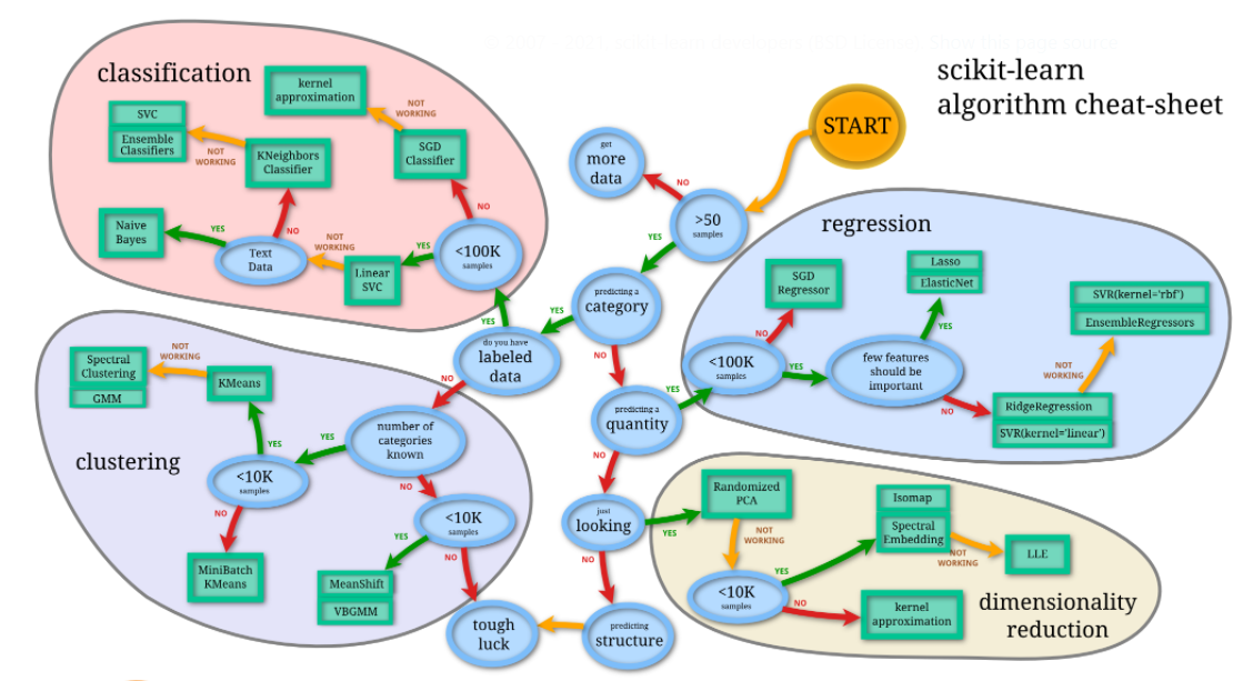
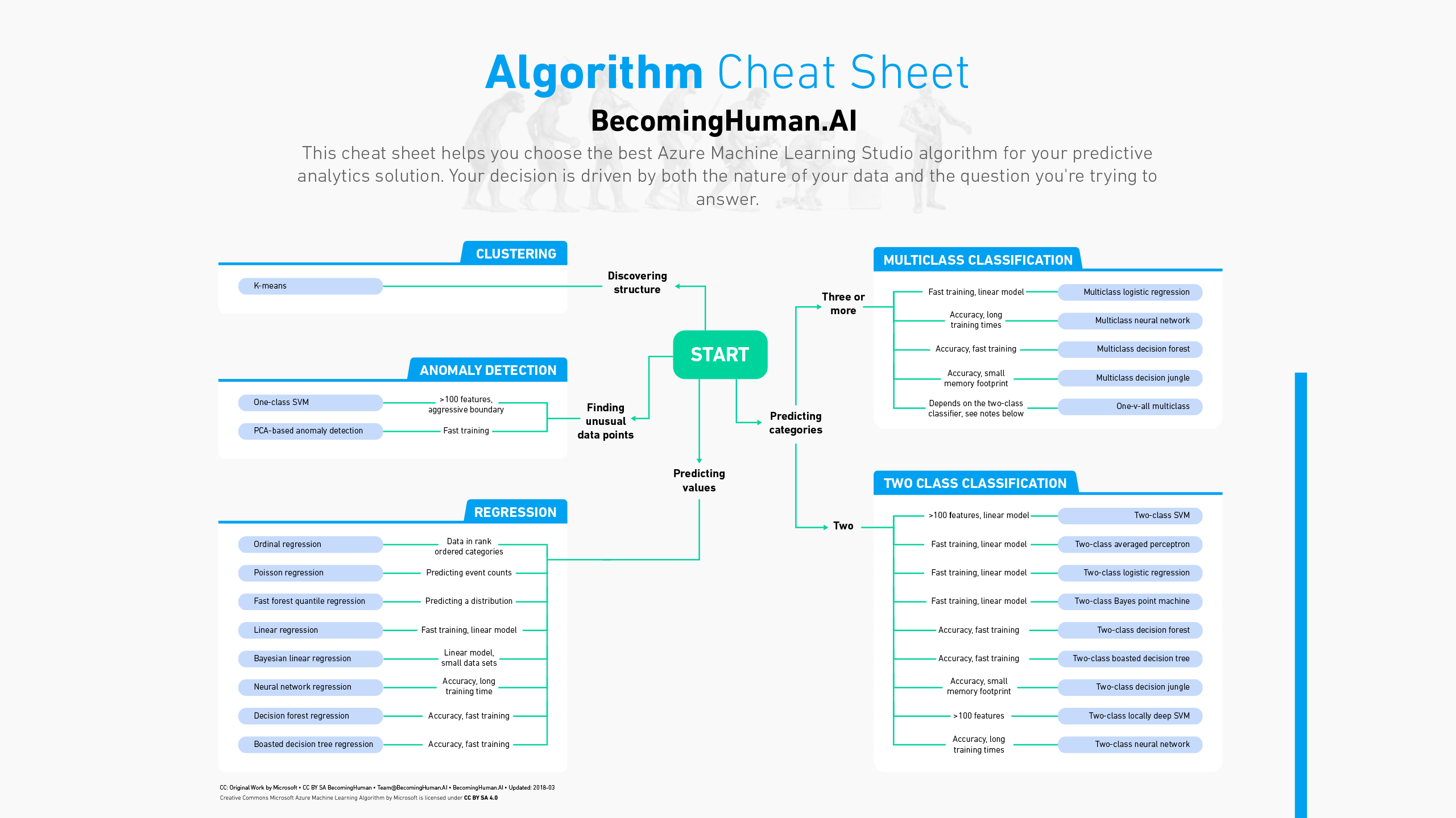
Observations:
The data cleaning step of a data focused on the text analysis, with few columns, is very different from a data with a lot of variables with numeric info. Thus, the algorithms we are going to use for machine learning may not be the ones we implement on a price prediction, for example.
Always good to remember this sheet:
from IPython.display import Image
XGB Classifier:
XGBoost is an algorithm that has recently been dominating applied machine learning and Kaggle competitions for structured or tabular data. XGBoost is an implementation of gradient boosted decision trees designed for speed and performance.
import xgboost as xg
from sklearn.model_selection import cross_val_score
import warnings
warnings.filterwarnings("ignore")

param = xg.XGBClassifier(max_depth = 5, n_estimators = 500,
                        learning_rate = 0.08, nthread = 10, colsample_bytree = 0.8, eval_metric = "logloss")

XGB_vector_score = cross_val_score(param, tr_v, df_train['target'],
                              cv=5, scoring='f1')
print("Vector score: ", XGB_vector_score)

XGB_tfidf_score = cross_val_score(param, tr_t, df_train['target'],
                              cv=5, scoring='f1')
print("\nTFIDF score: ", XGB_tfidf_score)
Vector score:  [0.50638298 0.40636704 0.49578415 0.40161453 0.56742557]

TFIDF score:  [0.49455338 0.39425837 0.48713551 0.40162272 0.57444934]
Logistic Regression:
There are lots of classification problems that are available, but the logistics regression is common and is an useful regression method for solving the binary classification problem.
from sklearn.linear_model import LogisticRegression

lg = LogisticRegression()
LR_vector_score = cross_val_score(lg, tr_v, df_train['target'],
                              cv=5, scoring='f1')
print("LR_Vector score: ", LR_vector_score)

LR_tfidf_score = cross_val_score(lg, tr_t, df_train['target'],
                              cv=5, scoring='f1')
print("\nLR_TFIDF score: ", LR_tfidf_score)
LR_Vector score:  [0.62655205 0.52433817 0.6035313  0.52847806 0.7057903 ]

LR_TFIDF score:  [0.5623069  0.5013876  0.56862745 0.42629905 0.67244367]
Naive Bayes:
Naive Bayes is the most straightforward and fast classification algorithm, which is suitable for a large chunk of data. Naive Bayes classifier is successfully used in various applications such as spam filtering, text classification, sentiment analysis, and recommender systems. It uses Bayes theorem of probability for prediction of unknown class.
from sklearn.naive_bayes import MultinomialNB as mb

m = mb()
NB_vector_score = cross_val_score(m, tr_v, df_train['target'],
                              cv=5, scoring='f1')
print("NB_Vector score: ", vector_score)

NB_tfidf_score = cross_val_score(m, tr_t, df_train['target'],
                              cv=5, scoring='f1')
print("\nNB_TFIDF score: ", tfidf_score)
NB_Vector score:  [0.64227642 0.61965812 0.67412587 0.6407465  0.73404255]

NB_TFIDF score:  [0.57838364 0.58523726 0.62139219 0.59797608 0.74842767]
Converting Score arrays to Data frames, I guess it’s better to plot
XGB_V = pd.DataFrame(XGB_vector_score,
             columns=['XGB_Vector Score'])

LR_V = pd.DataFrame(LR_vector_score,
             columns=['LR_Vector Score'])

NB_V = pd.DataFrame(NB_vector_score,
             columns=['NB_Vector Score'])

FULL_V = pd.concat([XGB_V ,LR_V, NB_V], axis=1, join="inner")
print("\n",FULL_V)
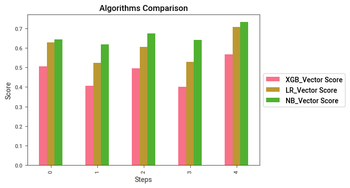
    XGB_Vector Score  LR_Vector Score  NB_Vector Score
0          0.506383         0.626552         0.642799
1          0.406367         0.524338         0.617249
2          0.495784         0.603531         0.674126
3          0.401615         0.528478         0.640125
4          0.567426         0.705790         0.732713
Plot the Vector scores to compare
FULL_V.plot(kind="bar").legend(loc='center left', bbox_to_anchor=(1, 0.5))
plt.title("Algorithms Comparison")
plt.xlabel("Steps")
plt.ylabel("Score")
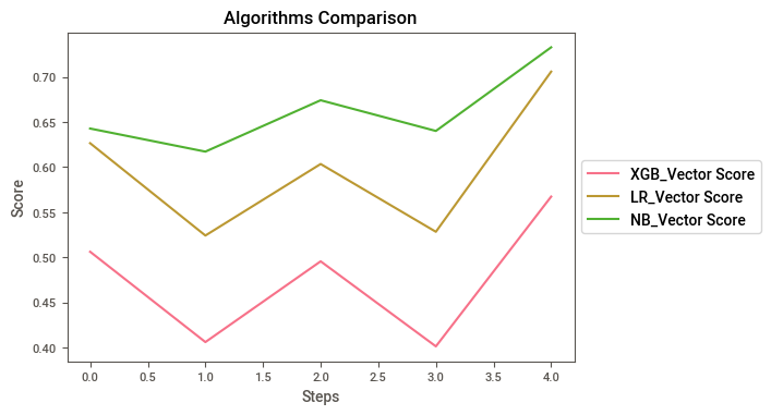
FULL_V.plot().legend(loc='center left', bbox_to_anchor=(1, 0.5))
plt.title("Algorithms Comparison")
plt.xlabel("Steps")
plt.ylabel("Score")
Text(0, 0.5, 'Score')
XGB_TFIDF = pd.DataFrame(XGB_tfidf_score,
             columns=['XGB_TF Score'])

LR_TFIDF = pd.DataFrame(LR_tfidf_score,
             columns=['LR_TFr Score'])

NB_TFIDF = pd.DataFrame(NB_tfidf_score,
             columns=['NB_TF Score'])

FULL_TF = pd.concat([XGB_TFIDF,LR_TFIDF,NB_TFIDF], axis=1, join="inner")
print("\n",FULL_TF)
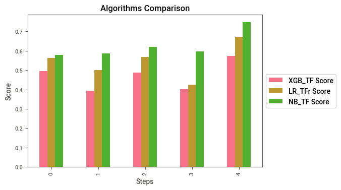
    XGB_TF Score  LR_TFr Score  NB_TF Score
0      0.494553      0.562307     0.578947
1      0.394258      0.501388     0.585237
2      0.487136      0.568627     0.621392
3      0.401623      0.426299     0.597976
4      0.574449      0.672444     0.748428
Plot the TFIDF scores to compare
FULL_TF.plot(kind="bar").legend(loc='center left', bbox_to_anchor=(1, 0.5))
plt.title("Algorithms Comparison")
plt.xlabel("Steps")
plt.ylabel("Score")

FULL_TF.plot().legend(loc='center left', bbox_to_anchor=(1, 0.5))
plt.title("Algorithms Comparison")
plt.xlabel("Steps")
plt.ylabel("Score")
Text(0, 0.5, 'Score')
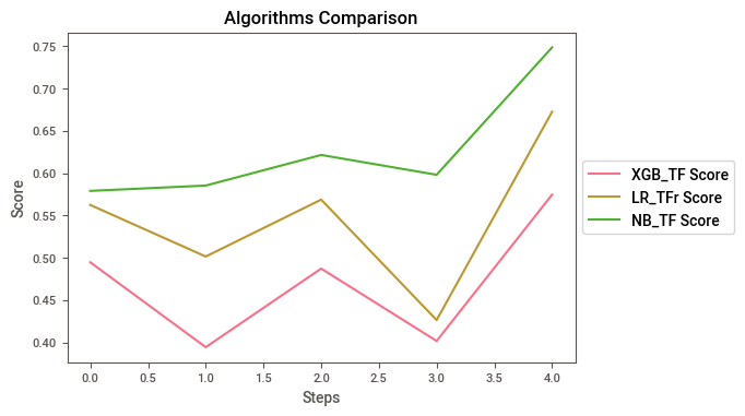
As we can see, Naive Bayes has the best results by far, so no we are going to submit.
Prediction
m.fit(tr_t,df_train['target'])
pred = m.predict(te_t)
Submission to Kaggle
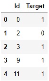
s = pd.DataFrame({'Id':df_test['id'],
                 'Target':pred})
s.to_csv('s.csv',index = False)
s = pd.read_csv('s.csv')
s.head(5)
And now we arrived to the end of our analysis. The next step would be the machine learning deployment and improvement of the models. I hope you enjoyed and learned something from this material. Thank you ༼ つ ◕_◕ ༽つ